Classification
The goal of classification is to leverage patterns in natural and social processes to conjecture about uncertain outcomes. An outcome may be uncertain because it lies in the future. This is the case when we try to predict whether a loan applicant will pay back a loan by looking at various characteristics such as credit history and income. Classification also applies to situations where the outcome has already occurred, but we are unsure about it. For example, we might try to classify whether financial fraud has occurred by looking at financial transactions.
What makes classification possible is the existence of patterns that connect the outcome of interest in a population to pieces of information that we can observe. Classification is specific to a population and the patterns prevalent in the population. Risky loan applicants might have a track record of high credit utilization. Financial fraud often coincides with irregularities in the distribution of digits in financial statements. These patterns might exist in some contexts but not others. As a result, the degree to which classification works varies.
We formalize classification in two steps. The first is to represent a population as a probability distribution. While often taken for granted in quantitative work today, the act of representing a dynamic population of individuals as a probability distribution is a significant shift in perspective. The second step is to apply statistics, specifically statistical decision theory, to the probability distribution that represents the population. Statistical decision theory formalizes the classification objective, allowing us to talk about the quality of different classifiers.
The statistical decision-theoretic treatment of classification forms the foundation of supervised machine learning. Supervised learning makes classification algorithmic in how it provides heuristics to turn samples from a population into good classification rules.
Modeling populations as probability distributions
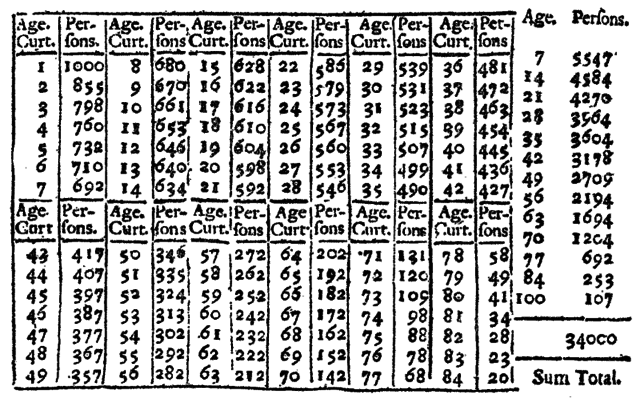
One of the earliest applications of probability to the study of human populations is Halley’s life table from 1693. Halley tabulated births and deaths in a small town in order to estimate life expectancy in the population. Estimates of life expectancy, then as novel as probability theory itself, found use in accurately pricing investments that paid an amount of money annually for the remainder of a person’s life.
For centuries that followed, the use of probability to model human populations, however, remained contentious both scientifically and politically.Alain Desrosières, The Politics of Large Numbers: A History of Statistical Reasoning (Harvard University Press, 1998); Theodore M Porter, The Rise of Statistical Thinking, 1820–1900 (Princeton University Press, 2020); Dan Bouk, How Our Days Became Numbered: Risk and the Rise of the Statistical Individual (University of Chicago Press, 2015). Among the first to apply statistics to the social sciences was the 19th astronomer and sociologist Adolphe Quetelet. In a scientific program he called “social physics”, Quetelet sought to demonstrate the existence of statistical laws in human populations. He introduced the concept of the “average man” characterized by the mean values of measured variables, such as height, that followed a normal distribution. As much a descriptive as a normative proposal, Quetelet regarded averages as an ideal to be pursued. Among others, his work influenced Francis Galton in the development of eugenics.
The success of statistics throughout the 20th century cemented in the use of probability to model human populations. Few raise an eyebrow today if we talk about a survey as sampling responses from a distribution. It seems obvious now that we’d like to estimate parameters such as mean and standard deviation from distributions of incomes, household sizes, or other such attributes. Statistics is so deeply embedded in the social sciences that we rarely revisit the premise that we can represent a human population as a probability distribution.
The differences between a human population and a distribution are stark. Human populations change over time, sometimes rapidly, due to different actions, mechanisms, and interactions among individuals. A distribution, in contrast, can be thought of as a static array where rows correspond to individuals and columns correspond to measured covariates of an individual. The mathematical abstraction for such an array is a set of nonnegative numbers, called probabilities, that sum up to 1 and give us for each row the relative weight of this setting of covariates in the population. To sample from such a distribution corresponds to picking one of the rows in the table at random in proportion to its weight. We can repeat this process without change or deterioration. In this view, the distribution is immutable. Nothing we do can change the population.
Much of statistics deals with samples and the question how we can relate quantities computed on a sample, such as the sample average, to corresponding parameters of a distribution, such as the population mean. The focus in our chapter is different. We’ll use statistics to talk about properties of populations as distributions and by extension classification rules applied to a population. While sampling introduces many additional issues, the questions we raise in this chapter come out most clearly at the population level.
Formalizing classification
The goal of classification is to determine a plausible value for an unknown target Y given observed covariates X. Typically, the covariates are represented as an an array of continuous or discrete variables, while the target is discrete, often binary, value. Formally, the covariates X and target Y are jointly distributed random variables. This means that there is one probability distribution over pairs of values (x,y) that the random variables (X,Y) might take on. This probability distribution models a population of instances of the classification problem. In most of our examples, we think of each instance as the covariates and target of one individual.
At the time of classification, the value of the target variable is not known to us, but we observe the covariates X and make a guess \hat Y = f(X) based on what we observed. The function f that maps our covariates into our guess \hat Y is called a classifier, or predictor. The output of the classifier is called label or prediction. Throughout this chapter we are primarily interested with the random variable \hat Y and how it relates to other random variables. The function that defines this random variables is secondary. For this reason, we stretch the terminology slightly and refer to \hat Y itself as the classifier.
Implicit in this formal setup of classification is a major assumption. Whatever we do on the basis of the covariates X cannot influence the outcome Y. After all, our distribution assigns a fixed weight to each pair (x,y). In particular, our prediction \hat Y cannot influence the outcome Y. This assumption is often violated when predictions motivate actions that influence the outcome. For example, the prediction that a student is at risk of dropout, might be followed with educational interventions that make dropout less likely.
To be able to choose a classifier out of many possibilities, we need to formalize what makes a classifier good. This question often does not have a fully satisfying answer, but statistical decision theory provides criteria that can help highlight different qualities of a classifier that can inform our choice.
Perhaps the most well known property of a classifier \hat Y is its classification accuracy, or accuracy for short, defined as \mathbb{P}\{Y=\hat Y\}, the probability of correctly predicting the target variable. We define classification error as \mathop\mathbb{P}\{Y\ne\hat Y\}. Accuracy is easy to define, but misses some important aspects when evaluating a classifier. A classifier that always predicts no traffic fatality in the next year might have high accuracy on any given individual, simply because fatal accidents are unlikely. However, it’s a constant function that has no value in assessing the risk of a traffic fatality.
Other decision-theoretic criteria highlight different aspects of a classifier. We can define the most common ones by considering the conditional probability \mathbb{P}\{\mathrm{event}\mid \mathrm{condition}\} for various different settings.
| Event | Condition | Resulting notion (\mathbb{P}\{\mathrm{event}\mid \mathrm{condition}\}) |
|---|---|---|
| \hat Y=1 | Y=1 | True positive rate, recall |
| \hat Y=0 | Y=1 | False negative rate |
| \hat Y=1 | Y=0 | False positive rate |
| \hat Y=0 | Y=0 | True negative rate |
The true positive rate corresponds to the frequency with which the classifier correctly assigns a positive label when the outcome is positive. We call this a true positive. The other terms false positive, false negative, and true negative derive analogously from the respective definitions. It is not important to memorize all these terms. They do, however, come up regularly in the classification settings.
Another family of classification criteria arises from swapping event and condition. We’ll only highlight two of the four possible notions.
| Event | Condition | Resulting notion (\mathbb{P}\{\mathrm{event}\mid\mathrm{condition}\}) |
|---|---|---|
| Y=1 | \hat Y=1 | Positive predictive value, precision |
| Y=0 | \hat Y=0 | Negative predictive value |
Optimal classification
Suppose we assign a quantified cost (or reward) to each of the four possible classification outcomes, true positive, false positive, true negative, false negative. The problem of optimal classification is to find a classifier that minimizes cost in expectation over a population. We can write the cost as a real number \ell(\hat y, y), called loss, that we experience when we classify a target value y with a label \hat y. An optimal classifier is any classifier that minimizes the expected loss: \mathop\mathbb{E}[\ell(\hat Y, Y)] This objective is called classification risk and risk minimization refers to the optimization problem of finding a classifier that minimizes risk.
As an example, choose the losses \ell(0,1)=\ell(1,0)=1 and \ell(1,1)=\ell(0,0)=0. For this choice of loss function, the optimal classifier is the one that minimizes classification error. The resulting optimal classifier has an intuitive solution.
The optimal predictor minimizing classification error satisfies \hat Y = f(X)\,,\quad\text{where}\quad f(x) = \begin{cases} 1 & \text{ if } \mathop\mathbb{P}\{ Y = 1\mid X=x\} > 1/2\\ 0 & \text{ otherwise.} \end{cases}
The optimal classifier checks if the propensity of positive outcomes given the observed covariates X is greater than 1/2. If so, it makes the guess that the outcome is 1. Otherwise, it guesses that the outcome is 0. The optimal predictor above is specific to classification error. If our loss function were different, the threshold 1/2 in the definition above would need to change. This makes intuitive sense. If our cost for false positives was much higher than our cost for false negatives, we’d better err on the side of not declaring a positive.
The optimal predictor is a theoretical construction that we may not be able to build from data. For example, when the vector of covariates X is high-dimensional, a finite sample is likely going to miss out on some settings X=x that the covariates might take on. In this case, it’s not clear how to get at the probability \mathop\mathbb{P}\{Y = 1\mid X=x\}. There is a vast technical repertoire in statistics and machine learning for finding good predictors from finite samples. Throughout this chapter we focus on problems that persist even if we had access to the optimal predictor for a given population.
Risk scores
The optimal classifier we just saw has an important property. We were able to write it as a threshold applied to the function r(x) = \mathop\mathbb{P}\{Y = 1\mid X=x\} = \mathop\mathbb{E}[Y\mid X=x]\,. This function is an example of a risk score. Statistical decision theory tells us that optimal classifiers can generally be written as a threshold applied to this risk score. The risk score we see here is a particularly important and natural one. We can think of it as taking the available evidence X=x and calculating the expected outcome given the observed information. This is called the posterior probability of the outcome Y given X. In an intuitive sense, the conditional expectation is a statistical lookup table that gives us for each setting of features the frequency of positive outcomes given these features. The risk score is sometimes called Bayes optimal. It minimizes the squared loss \mathop\mathbb{E}(Y-r(X))^2 among all possible real-valued risk scores r(X). Minimization problems where we try to approximate the target variable Y with a real-valued risk score are called regression problems. In this context, risk scores are often called regressors. Although our loss function was specific, there is a general lesson. Classification is often attacked by first solving a regression problem to summarize the data in a single real-valued risk score. We then turn the risk score into a classifier by thresholding.
Risk scores need not be optimal or learned from data. For an illustrative example consider the well-known body mass index, due to Quetelet by the way, which summarizes weight and height of a person into a single real number. In our formal notation, the features are X=(H, W) where H denotes height in meters and W denotes weight in kilograms. The body mass index corresponds to the score function R=W/H^2.

We could interpret the body mass index as measuring risk of, say, diabetes. Thresholding it at the value 30, we might decide that individuals with a body mass index above this value are at risk of developing diabetes while others are not. It does not take a medical degree to worry that the resulting classifier may not be very accurate. The body mass index has a number of known issues leading to errors when used for classification. We won’t go into detail, but it’s worth noting that these classification errors can systematically align with certain groups in the population. For instance, the body mass index tends to be inflated as a risk measure for taller people due to scaling issues.
A more refined approach to finding a risk score for diabetes would be to solve a regression problem involving the available covariates and the outcome variable. Solved optimally, the resulting risk score would tell us for every setting of weight (say, rounded to the nearest kg unit) and every physical height (rounded to the nearest cm unit), the incidence rate of diabetes among individuals with these values of weight and height. The target variable in this case is a binary indicator of diabetes. So, r((176, 68)) would be the incidence rate of diabetes among individuals who are 1.76m tall and weigh 68kg. The conditional expectation is likely more useful as a risk measure of diabetes than the body mass index we saw earlier. After all, the conditional expectation directly reflects the incidence rate of diabetes given the observed characteristics, while the body mass index didn’t solve this specific regression problem.
Varying thresholds and ROC curves
In the optimal predictor for classification error we chose a threshold of 1/2. This exact number was a consequence of the equal cost for false positives and false negatives. If a false positive was significantly more costly, we might wish to choose a higher threshold for declaring a positive. Each choice of a threshold results in a specific trade-off between true positive rate and false positive rate. By varying the threshold from 0 to 1, we can trace out a curve in a two-dimensional space where the axes correspond to true positive rate and false positive rate. This curve is called an ROC curve. ROC stands for receiver operator characteristic, a name pointing at the roots of the concept in signal processing.

In statistical decision theory, the ROC curve is a property of a distribution (X, Y). It gives us for each setting of false positive rate, the optimal true positive rate that can be achieved for the given false positive rate on the distribution (X, Y). This leads to several nice theoretical properties of the ROC curve. In the machine learning context, ROC curves are computed more liberally for any given risk score, even if it isn’t optimal. The ROC curve is often used to eyeball how predictive our score is of the target variable. A common measure of predictiveness is the area under the curve (AUC), which equals the probability that a random positive instance gets a score higher than a random negative instance. An area of 1/2 corresponds to random guessing, and an area of 1 corresponds to perfect classification.
Supervised learning
Supervised learning is what makes classification algorithmic. It’s about how to construct good classifiers from samples drawn from a population. The details of supervised learning won’t matter for this chapter, but it is still worthwhile to have a working understanding of the basic idea.
Suppose we have labeled data, also called training examples, of the form (x_1,y_1), ..., (x_n, y_n), where each example is a pair (x_i,y_i) of an instance x_i and a label y_i. We typically assume that these examples were drawn independently and repeatedly from the same distribution (X, Y). A supervised learning algorithm takes in training examples and returns a classifier, typically a threshold of a score: f(x)=\mathbb{1}\{r(x) > t\}. A simple example of a learning algorithm is the familiar least squares method that attempts to minimize the objective function \sum_{i=1}^n \left(r(x_i)-y_i\right)^2\,. We saw earlier that at the population level, the optimal score is the conditional expectation r(x)=\mathbb{E}\left[Y\mid X=x\right]. The problem is that we don’t necessarily have enough data to estimate each of the conditional probabilities required to construct this score. After all, the number of possible values that x can assume is exponential in the number of covariates.
The whole trick in supervised learning is to approximate this optimal solution with algorithmically feasible solutions. In doing so, supervised learning must negotiate a balance along three axes:
- Representation: Choose a family of functions that the score r comes from. A common choice are linear functions r(x) = \langle w, x\rangle that take the inner product of the covariates x with some vector of coefficients w. More complex representations involve non-linear functions, such as artificial neural networks. This function family is often called the model class and the coefficients w are called model parameters.
- Optimization: Solve the resulting optimization problem by finding model parameters that minimize the loss function on the training examples.
- Generalization: Ensure that small loss on the training examples implies small loss on the population that we drew the training examples from.
The three goals of supervised learning are entangled. A powerful representation might make it easier to express complicated patterns, but it might also burden optimization and generalization. Likewise, there are tricks to make optimization feasible at the expense of representation or generalization.
For the remainder of this chapter, we can think of supervised learning as a black box that provides us with classifiers when given labeled training data. What matters are which properties these classifiers have at the population level. At the population level, we interpret a classifier as a random variable by considering \hat Y=f(X). We ignore how \hat Y was learned from a finite sample, what the functional form of the classifier is, and how we estimate various statistical quantities from finite samples. While finite sample considerations are fundamental to machine learning, they are not central to the conceptual and technical questions around fairness that we will discuss in this chapter.
Groups in the population
Chapter 2 introduced some of the reasons why individuals might want to object to the use of statistical classification rules in consequential decisions. We now turn to one specific concern, namely, discrimination on the basis of membership in specific groups of the population. Discrimination is not a general concept. It is concerned with socially salient categories that have served as the basis for unjustified and systematically adverse treatment in the past. United States law recognizes certain protected categories including race, sex (which extends to sexual orientation), religion, disability status, and place of birth.
In many classification tasks, the features X implicitly or explicitly encode and individual’s status in a protected category. We will set aside the letter A to designate a discrete random variable that captures one or multiple sensitive characteristics. Different settings of the random variable A correspond to different mutually disjoint groups of the population. The random variable A is often called a sensitive attribute in the technical literature.
Note that formally we can always represent any number of discrete protected categories as a single discrete attribute whose support corresponds to each of the possible settings of the original attributes. Consequently, our formal treatment in this chapter does apply to the case of multiple protected categories. This formal maneuver, however, does not address the important concept of intersectionality that refers to the unique forms of disadvantage that members of multiple protected categories may experience.Kimberlé W Crenshaw, On Intersectionality: Essential Writings (The New Press, 2017).
The fact that we allocate a special random variable for group membership does not mean that we can cleanly partition the set of features into two independent categories such as “neutral” and “sensitive”. In fact, we will see shortly that sufficiently many seemingly neutral features can often give high accuracy predictions of group membership. This should not be surprising. After all, if we think of A as the target variable in a classification problem, there is reason to believe that the remaining features would give a non-trivial classifier for A.
The choice of sensitive attributes will generally have profound consequences as it decides which groups of the population we highlight, and what conclusions we draw from our investigation. The taxonomy induced by discretization can on its own be a source of harm if it is too coarse, too granular, misleading, or inaccurate. The act of classifying status in protected categories, and collecting associated data, can on its own can be problematic. We will revisit this important discussion in the next chapter.
No fairness through unawareness
Some have hoped that removing or ignoring sensitive attributes would somehow ensure the impartiality of the resulting classifier. Unfortunately, this practice can be ineffective and even harmful.
In a typical dataset, we have many features that are slightly
correlated with the sensitive attribute. Visiting the website
pinterest.com in the United States, for example, had at the
time of writing a small statistical correlation with being female. The
correlation on its own is too small to classify someone’s gender with
high accuracy. However, if numerous such features are available, as is
the case in a typical browsing history, the task of classifying gender
becomes feasible at higher accuracy levels.

Several features that are slightly predictive of the sensitive attribute can be used to build high accuracy classifiers for that attribute. In large feature spaces sensitive attributes are generally redundant given the other features. If a classifier trained on the original data uses the sensitive attribute and we remove the attribute, the classifier will then find a redundant encoding in terms of the other features. This results in an essentially equivalent classifier, in the sense of implementing the same function.
To further illustrate the issue, consider a fictitious start-up that sets out to predict your income from your genome. At first, this task might seem impossible. How could someone’s DNA reveal their income? However, we know that DNA encodes information about ancestry, which in turn correlates with income in some countries such as the United States. Hence, DNA can likely be used to predict income better than random guessing. The resulting classifier uses ancestry in an entirely implicit manner. Removing redundant encodings of ancestry from the genome is a difficult task that cannot be accomplished by removing a few individual genetic markers. What we learn from this is that machine learning can wind up building classifiers for sensitive attributes without explicitly being asked to, simply because it is an available route to improving accuracy.
Redundant encodings typically abound in large feature spaces. For example, gender can be predicted from retinal photographs with very high accuracy.Ryan Poplin et al., “Prediction of Cardiovascular Risk Factors from Retinal Fundus Photographs via Deep Learning,” Nature Biomedical Engineering 2, no. 3 (2018): 158–64. What about small hand-curated feature spaces? In some studies, features are chosen carefully so as to be roughly statistically independent of each other. In such cases, the sensitive attribute may not have good redundant encodings. That does not mean that removing it is a good idea. Medication, for example, sometimes depends on race in legitimate ways if these correlate with underlying causal factors.Vence L Bonham, Shawneequa L Callier, and Charmaine D Royal, “Will Precision Medicine Move Us Beyond Race?” The New England Journal of Medicine 374, no. 21 (2016): 2003. Forcing medications to be uncorrelated with race in such cases can harm the individual.
Statistical non-discrimination criteria
Statistical non-discrimination criteria aim to define the absence of
discrimination in terms of statistical expressions involving random
variables describing a classification or decision making scenario.
Formally, statistical non-discrimination criteria are properties of the
joint distribution of the sensitive attribute A, the target variable Y, the classifier \hat Y or score R, and in some cases also features X. This means that we can unambiguously
decide whether or not a criterion is satisfied by looking at the joint
distribution of these random variables.
Broadly speaking, different statistical fairness criteria all equalize some group-dependent statistical quantity across groups defined by the different settings of A. For example, we could ask to equalize acceptance rates across all groups. This corresponds to imposing the constraint for all groups a and b: \mathbb{P}\{\hat Y = 1 \mid A=a\} = \mathop\mathbb{P}\{\hat Y=1 \mid A=b\}\,. In the case where \hat Y\in\{0, 1\} is a binary classifier and we have two groups a and b, we can determine if acceptance rates are equal in both groups by knowing the three probabilities \mathbb{P}\{\hat Y=1, A=a\}, \mathbb{P}\{\hat Y=1,A=b\}, and \mathbb{P}\{A=a\} that fully specify the joint distribution of \hat Y and A. We can also estimate the relevant probabilities given random samples from the joint distribution using standard statistical arguments that are not the focus of this chapter.
Researchers have proposed dozens of different criteria, each trying to capture different intuitions about what is fair. Simplifying the landscape of fairness criteria, we can say that there are essentially three fundamentally different ones. Each of these equalizes one of the following three statistics across all groups:
- Acceptance rate \mathop\mathbb{P}\{\hat Y = 1\} of a classifier \hat Y
- Error rates \mathop\mathbb{P}\{\hat Y = 0 \mid Y = 1\} and \mathop\mathbb{P}\{\hat Y = 1 \mid Y =0\} of a classifier \hat Y
- Outcome frequency given score value \mathop\mathbb{P}\{Y = 1 \mid R = r\} of a score R
The three criteria can be generalized to score functions using simple (conditional) independence statements. We use the notation U\bot V\mid W to denote that random variables U and V are conditionally independent given W. This means that conditional on any setting W=w, the random variables U and V are independent.
| Independence | Separation | Sufficiency |
|---|---|---|
| R\bot A | R\bot A \mid Y | Y\bot A\mid R |
Below we will introduce and discuss each of these conditions in detail. This chapter focuses on the mathematical properties of and relationships between these different criteria. Once we have acquired familiarity with the technical matter, we’ll have a broader debate around the moral and normative content of these definitions in Chapter 4.
Independence
Our first formal criterion requires the sensitive characteristic to be statistically independent of the score.
Random variables (A, R) satisfy independence if A\bot R.
If R is a score function that satisfies independence, then any classifier \hat Y = \mathbb{1}\{R > t\} that thresholds the score a value t also satisfies independence. This is true so long as the threshold is independent of group membership. Group-specific thresholds may not preserve independence.
Independence has been explored through many equivalent and related definitions. When applied to a binary classifier \hat Y, independence is often referred to as demographic parity, statistical parity, group fairness, disparate impact and others. In this case, independence corresponds to the condition \mathbb{P}\{\hat Y =1\mid A=a\}=\mathbb{P}\{\hat Y=1\mid A=b\}\,, for all groups a, b. Thinking of the event \hat Y=1 as “acceptance”, the condition requires the acceptance rate to be the same in all groups. A relaxation of the constraint introduces a positive amount of slack \epsilon>0 and requires that \mathbb{P}\{\hat Y=1\mid A=a\}\ge \mathbb{P}\{\hat Y=1\mid A=b\}-\epsilon\,.
Note that we can swap a and b to get an inequality in the other direction. An alternative relaxation is to consider a ratio condition, such as, \frac{\mathbb{P}\{\hat Y=1\mid A=a\}} {\mathbb{P}\{\hat Y=1\mid A=b\}}\ge1-\epsilon\,. Some have argued that, for \epsilon=0.2, this condition relates to the 80 percent rule that appears in discussions around disparate impact law.Michael Feldman et al., “Certifying and Removing Disparate Impact,” in Proc. 21St SIGKDD (ACM, 2015).
Yet another way to state the independence condition in full generality is to require that A and R must have zero mutual information I(A;R)=0. Mutual information quantifies the amount of information that one random variable reveals about the other. We can define it in terms of the more standard entropy function as I(A;R)=H(A)+H(R)-H(A,R). The characterization in terms of mutual information leads to useful relaxations of the constraint. For example, we could require I(A;R)\le\epsilon.
Limitations of independence
Independence is pursued as a criterion in many papers, for multiple reasons. Some argue that the condition reflects an assumption of equality: All groups have an equal claim to acceptance and resources should therefore be allocated proportionally. What we encounter here is a question about the normative significance of independence, which we extend on in Chapter 4. But there is a more mundane reason for the prevalence of this criterion, too. Independence has convenient technical properties, which makes the criterion appealing to machine learning researchers. It is often the easiest one to work with mathematically and algorithmically.
However, decisions based on a classifier that satisfies independence can have undesirable properties (and similar arguments apply to other statistical criteria). Here is one way in which this can happen, which is easiest to illustrate if we imagine a callous or ill-intentioned decision maker. Imagine a company that in group a hires diligently selected applicants at some rate p>0. In group b, the company hires carelessly selected applicants at the same rate p. Even though the acceptance rates in both groups are identical, it is far more likely that unqualified applicants are selected in one group than in the other. As a result, it will appear in hindsight that members of group b performed worse than members of group a, thus establishing a negative track record for group b.
A real-world phenomenon similar to this hypothetical example is termed the glass cliff: women and people of color are more likely to be appointed CEO when a firm is struggling. When the firm performs poorly during their tenure, they are likely to be replaced by White men.Michelle K Ryan and S Alexander Haslam, “The Glass Cliff: Evidence That Women Are over-Represented in Precarious Leadership Positions,” British Journal of Management 16, no. 2 (2005): 81–90; Alison Cook and Christy Glass, “Above the Glass Ceiling: When Are Women and Racial/Ethnic Minorities Promoted to CEO?” Strategic Management Journal 35, no. 7 (2014): 1080–89.
This situation might arise without positing malice: the company might have historically hired employees primarily from group a, giving them a better understanding of this group. As a technical matter, the company might have substantially more training data in group a, thus potentially leading to lower error rates of a learned classifier within that group. The last point is a bit subtle. After all, if both groups were entirely homogeneous in all ways relevant to the classification task, more training data in one group would equally benefit both. Then again, the mere fact that we chose to distinguish these two groups indicates that we believe they might be heterogeneous in relevant aspects.
Separation
Our next criterion engages with the limitation of independence that we described. In a typical classification problem, there is a difference between accepting a positive instance or accepting a negative instance. The target variable Y suggests one way of partitioning the population into strata of equal claim to acceptance. Viewed this way, the target variable gives us a sense of merit. A particular demographic group (A=a) may be more or less well represented in these different strata defined by the target variable. A decision maker might argue that in such cases it is justified to accept more or fewer individuals from group a.
These considerations motivate a criterion that demands independence within each stratum of the population defined by target variable. We can formalize this requirement using a conditional independence statement.
Random variables (R, A, Y) satisfy separation if R\bot A \mid Y.
The conditional independence statement applies even if the variables take on more than two values each. For example, the target variable might partition the population into many different types of individuals.
We can display separation as a graphical model in which R is separated from A by the target variable Y:

If you haven’t seen graphical models before, don’t worry. All this says is that R is conditionally independent of A given Y.
In the case of a binary classifier, separation is equivalent to requiring for all groups a,b the two constraints \begin{aligned} \mathbb{P}\{ \hat Y=1 \mid Y=1, A=a\} &= \mathbb{P}\{ \hat Y=1 \mid Y=1, A=b\}\\ \mathbb{P}\{ \hat Y=1 \mid Y=0, A=a\} &= \mathbb{P}\{ \hat Y=1 \mid Y=0, A=b\}\,. \end{aligned}
Recall that \mathbb{P}\{\hat Y=1 \mid Y=1\} is called the true positive rate of the classifier. It is the rate at which the classifier correctly recognizes positive instances. The false positive rate \mathbb{P}\{\hat Y=1 \mid Y=0\} highlights the rate at which the classifier mistakenly assigns positive outcomes to negative instances. Recall that the true positive rate equals 1 minus the false negative rate. What separation therefore requires is that all groups experience the same false negative rate and the same false positive rate. Consequently, the definition asks for error rate parity.
This interpretation in terms of equality of error rates leads to natural relaxations. For example, we could only require equality of false negative rates. A false negative, intuitively speaking, corresponds to denied opportunity in scenarios where acceptance is desirable, such as in hiring. In contrast, when the task is to identify high-risk individuals, as in the case of loan default prediction, it is common to denote the undesirable outcome as the “positive” class. This inverts the meaning of false positives and false negatives, and is a frequent source of terminological confusion.
Why equalize error rates?
The idea of equalizing error rates across has been subject to critique. Much of the debate has to do with the fact that an optimal predictor need not have equal error rates in all groups. Specifically, when the propensity of positive outcomes (\mathbb{P}\{Y=1\}) differs between groups, an optimal predictor will generally have different error rates. In such cases, enforcing equality of error rates leads to a predictor that performs worse in some groups than it could be. How is that fair?
One response is that separation puts emphasis on the question: Who bears the cost of misclassification? A violation of separation highlights the fact that different groups experience different costs of misclassification. There is concern that higher error rates coincide with historically marginalized and disadvantaged groups, thus inflicting additional harm on these groups.
The act of measuring and reporting group specific error rates can create an incentive for decision makers to work toward improving error rates through collecting better datasets and building better models. If there is no way to improve error rates in some group relative to others, this raises questions about the legitimate use of machine learning in such cases. We will return to this normative question in later chapters.
A second line of concern with the separation criterion relates to the use of the target variable as a stand-in for merit. Researchers have rightfully pointed out that in many cases machine learning practitioners use target variables that reflect existing inequality and injustice. In such cases, satisfying separation with respect to an inadequate target variable does no good. This valid concern, however, applies equally to the use of supervised learning at large in such cases. If we cannot agree on an adequate target variable, the right action may be to suspend the use of supervised learning.
These observations hint at the subtle role that non-discrimination criteria play. Rather than presenting constraints that we can optimize for without further thought, they can help surface issues with the use of machine learning in specific scenarios.
Visualizing separation
A binary classifier that satisfies separation must achieve the same true positive rates and the same false positive rates in all groups. We can visualize this condition by plotting group-specific ROC curves.

We see the ROC curves of a score displayed for each group separately. The two groups have different curves indicating that not all trade-offs between true and false positive rate are achievable in both groups. The trade-offs that are achievable in both groups are precisely those that lie under both curves, corresponding to the intersection of the regions enclosed by the curves.

The highlighted region is the feasible region of trade-offs that we can achieve in all groups. However, the thresholds that achieve these trade-offs are in general also group-specific. In other words, the bar for acceptance varies by group. Trade-offs that are not exactly on the curves, but rather in the interior of the region, require randomization. To understand this point, think about how we can realize trade-offs on the the dashed line in the plot. Take one classifier that accepts everyone. This corresponds to true and false positive rate 1, hence achieving the upper right corner of the plot. Take another classifier that accepts no one, resulting in true and false positive rate 0, the lower left corner of the plot. Now, construct a third classifier that given an instance randomly picks and applies the first classifier with probability 1-p, and the second with probability p. This classifier achieves true and false positive rate p thus giving us one point on the dashed line in the plot. In the same manner, we could have picked any other pair of classifiers and randomized between them. This way we can realize the entire area under the ROC curve.
Conditional acceptance rates
A relative of the independence and separation criteria is common in debates around discrimination. Here, we designate a random variable W and ask for conditional independence of the decision \hat Y and group status A conditional on the variable W. That is, for all values w that W could take on, and all groups a and b we demand: \mathop\mathbb{P}\{\hat Y = 1 \mid W=w, A=a\} = \mathop\mathbb{P}\{\hat Y = 1 \mid W=w, A=b\} Formally, this is equivalent to replacing Y with W in our definition of separation. Often W corresponds to a subset of the covariates of X. For example, we might demand that independence holds among all individuals of equal educational attainment. In this case, we would choose W to reflect educational attainment. In doing so, we license the decision maker to distinguish between individuals with different educational backgrounds. When we apply this criterion, the burden falls on the proper choice of what to condition on, which determines whether we detect discrimination or not. In particular, we must be careful not to condition on the mechanism by which the decision maker discriminates. For example, an ill-intentioned decision maker might discriminate by imposing excessive educational requirements for a specific job, exploiting that this level of education is distributed unevenly among different groups. We will be able to return to the question of what to condition on with significantly more substance once we reach familiarity with causality in Chapter 5.
Sufficiency
Our third criterion formalizes that the score already subsumes the sensitive characteristic for the purpose of predicting the target. This idea again boils down to a conditional independence statement.
We say the random variables (R, A, Y) satisfy sufficiency if Y\bot A \mid R.
We can display sufficiency as a graphical model as we did with separation before.

Let us write out the definition more explicitly in the binary case where Y\in\{0,1\}. In this case, a random variable R is sufficient for A if and only if for all groups a,b and all values r in the support of R, we have \mathbb{P}\{Y=1 \mid R=r, A=a\}=\mathbb{P}\{ Y=1 \mid R=r, A=b\}\,. If we replace R by a binary predictor \hat Y, we recognize this condition as requiring a parity of positive/negative predictive values across all groups.
Calibration and sufficiency
Sufficiency is closely related to an important notion called calibration. In some applications it is desirable to be able to interpret the values of the score functions as if they were probabilities. The notion of calibration allows us to move in this direction. Restricting our attention to binary outcome variables, we say that a score R is calibrated with respect to an outcome variable Y if for all score values r\in[0,1], we have \mathbb{P}\{Y=1 \mid R=r\} = r\,. This condition means that the set of all instances assigned a score value r has an r fraction of positive instances among them. The condition refers to the group of all individuals receiving a particular score value. Calibration need not hold in subgroups of the population. In particular, it’s important not to interpret the score as an individual probability. Calibration does not tell us anything about the outcome of a specific individual that receives a particular value.
From the definition, we can see that sufficiency is closely related to the idea of calibration. To formalize the connection we say that the score R satisfies calibration by group if it satisfies \mathbb{P}\{Y=1 \mid R=r, A=a\} = r\,, for all score values r and groups a. Observe that calibration is the same requirement at the population level without the conditioning on A.
Calibration by group implies sufficiency.
Conversely, sufficiency is only slightly weaker than calibration by group in the sense that a simple renaming of score values goes from one property to the other.
If a score R satisfies sufficiency, then there exists a function \ell\colon[0,1]\to[0,1] so that \ell(R) satisfies calibration by group.
Fix any group a and put \ell(r) = \mathbb{P}\{Y=1\mid R=r, A=a\}. Since R satisfies sufficiency, this probability is the same for all groups a and hence this map \ell is the same regardless of what value a we chose.
Now, consider any two groups a,b. We have, \begin{aligned} r &= \mathbb{P}\{Y=1\mid \ell(R)=r, A=a\} \\ &= \mathbb{P}\{Y=1\mid R\in \ell^{-1}(r), A=a\} \\ &= \mathbb{P}\{Y=1\mid R\in \ell^{-1}(r), A=b\} \\ &= \mathbb{P}\{Y=1\mid \ell(R)=r, A=b\}\,,\end{aligned} thus showing that \ell(R) is calibrated by group.
We conclude that sufficiency and calibration by group are essentially equivalent notions.
In practice, there are various heuristics to achieve calibration. For example, Platt scaling takes a possibly uncalibrated score, treats it as a single feature, and fits a one variable regression model against the target variable based on this feature.John Platt et al., “Probabilistic Outputs for Support Vector Machines and Comparisons to Regularized Likelihood Methods,” Advances in Large Margin Classifiers 10, no. 3 (1999): 61–74. We also apply Platt scaling for each of the groups defined by the sensitive attribute.
Calibration by group as a consequence of unconstrained learning
Sufficiency is often satisfied by the outcome of unconstrained supervised learning without the need for any explicit intervention. This should not come as a surprise. After all, the goal of supervised learning is to approximate an optimal score function. The optimal score function we saw earlier, however, is calibrated for any group as the next fact states formally.
The optimal score r(x) = \mathbb{E}[ Y \mid X=x] satisfies group calibration for any group. Specifically, for any set S we have \mathbb{P}\{Y=1\mid R=r, X\in S\}=r.
We generally expect a learned score to satisfy sufficiency in cases where the group membership is either explicitly encoded in the data or can be predicted from the other attributes. To illustrate this point we look at the calibration values of a standard machine learning model, a random forest ensemble, on an income classification task derived from the American Community Survey of the US Census Bureau.Frances Ding et al., “Retiring Adult: New Datasets for Fair Machine Learning,” Advances in Neural Information Processing Systems 34 (2021). We restrict the dataset to the three most populous states, California, Texas, and Florida.
After splitting the data into training and testing data, we fit a random forest ensemble using the standard Python library sklearn on the training data. We then examine how well-calibrated the model is out of the box on test data.

We see that the calibration curves for the three largest racial groups in the dataset, which the Census Bureau codes as “White alone”, “Black or African American alone”, and “Asian alone”, are very close to the main diagonal. This means that the scores derived from our random forest model satisfy calibration by group up to small error. The same is true when looking at the two groups “Male” and “Female” in the dataset.
These observations are no coincidence. Theory shows that under certain technical conditions, unconstrained supervised learning does, in fact, imply group calibration.Lydia T Liu, Max Simchowitz, and Moritz Hardt, “The Implicit Fairness Criterion of Unconstrained Learning,” in International Conference on Machine Learning (PMLR, 2019), 4051–60. Note, however, that for this to be true the classifier must be able to detect group membership. If detecting group membership is impossible, then group calibration generally fails.
The lesson is that sufficiency often comes for free (at least approximately) as a consequence of standard machine learning practices. The flip side is that imposing sufficiency as a constraint on a classification system may not be much of an intervention. In particular, it would not effect a substantial change in current practices.
How to satisfy a non-discrimination criterion
Now that we have formally introduced three non-discrimination criteria, it is worth asking how we can achieve them algorithmically. We distinguish between three different techniques. While they generally apply to all the criteria and their relaxations that we review in this chapter, our discussion here focuses on independence.
- Pre-processing: Adjust the feature space to be uncorrelated with the sensitive attribute.
- In-training: Work the constraint into the optimization process that constructs a classifier from training data.
- Post-processing: Adjust a learned classifier so as to be uncorrelated with the sensitive attribute.
The three approaches have different strengths and weaknesses.
Pre-processing is a family of techniques to transform a feature space into a representation that as a whole is independent of the sensitive attribute. This approach is generally agnostic to what we do with the new feature space in downstream applications. After the pre-processing transformation ensures independence, any deterministic training process on the new space will also satisfy independence. This is a formal consequence of the well-known data processing inequality from information theory.Thomas M Cover, Elements of Information Theory (John Wiley & Sons, 1999).
Achieving independence at training time can lead to the highest utility since we get to optimize the classifier with this criterion in mind. The disadvantage is that we need access to the raw data and training pipeline. We also give up a fair bit of generality as this approach typically applies to specific model classes or optimization problems.
Post-processing refers to the process of taking a trained classifier and adjusting it possibly depending on the sensitive attribute and additional randomness in such a way that independence is achieved. Formally, we say a derived classifier \hat Y = F(R, A) is a possibly randomized function of a given score R and the sensitive attribute. Given a cost for false negatives and false positives, we can find the derived classifier that minimizes the expected cost of false positive and false negatives subject to the fairness constraint at hand. Post-processing has the advantage that it works for any black-box classifier regardless of its inner workings. There’s no need for re-training, which is useful in cases where the training pipeline is complex. It’s often also the only available option when we have access only to a trained model with no control over the training process.
Post-processing sometimes even comes with an optimality guarantee: If we post-process the Bayes optimal score to achieve separation, then the resulting classifier will be optimal among all classifiers satisfying separation.Moritz Hardt, Eric Price, and Nati Srebro, “Equality of Opportunity in Supervised Learning,” in Advances in Neural Information Processing Systems, 2016, 3315–23. Conventional wisdom has it that certain machine learning models, like gradient boosted decision trees, are often nearly Bayes optimal on tabular datasets with many more rows than columns. In such cases, post-processing by adjusting thresholds is nearly optimal.
A common objection to post-processing, however, is that the resulting classifier uses group membership quite explicitly by setting different acceptance thresholds for different groups.
Relationships between criteria
The criteria we reviewed constrain the joint distribution in non-trivial ways. We should therefore suspect that imposing any two of them simultaneously over-constrains the space to the point where only degenerate solutions remain. We will now see that this intuition is largely correct. What this shows, in particular, is that if we observe that one criterion holds, we expect others to be violated.
Independence versus sufficiency
We begin with a simple proposition that shows how in general independence and sufficiency are mutually exclusive. The only assumption needed here is that the sensitive attribute A and the target variable Y are not independent. This is a different way of saying that group membership has an effect on the statistics of the target variable. In the binary case, this means one group has a higher rate of positive outcomes than another. Think of this as the typical case.
Assume that A and Y are not independent. Then sufficiency and independence cannot both hold.
By the contraction rule for conditional independence, A\bot R \quad\mathrm{and}\quad A\bot Y \mid R \quad\Longrightarrow\quad A\bot (Y, R) \quad\Longrightarrow\quad A\bot Y\,. To be clear, A\bot (Y, R) means that A is independent of the pair of random variables (Y,R). Dropping R cannot introduce a dependence between A and Y.
In the contrapositive, A\not\bot Y \quad\Longrightarrow\quad A\not\bot R \quad\mathrm{or}\quad A\not\bot Y \mid A\,.
Independence versus separation
An analogous result of mutual exclusion holds for independence and separation. The statement in this case is a bit more contrived and requires the additional assumption that the target variable Y is binary. We also additionally need that the score is not independent of the target. This is a rather mild assumption, since any useful score function should have correlation with the target variable.
Assume Y is binary, A is not independent of Y, and R is not independent of Y. Then, independence and separation cannot both hold.
Assume Y\in\{0,1\}. In its contrapositive form, the statement we need to show is
A\bot R \quad\mathrm{and}\quad A\bot R \mid Y \quad\Longrightarrow\quad A\bot Y \quad\mathrm{or}\quad R\bot Y
By the law of total probability,
\mathbb{P}\{R=r\mid A=a\} =\sum_y \mathbb{P}\{R=r\mid A=a, Y=y\}\mathbb{P}\{Y=y\mid A=a\}
Applying the assumption A\bot R and A\bot R\mid Y, this equation simplifies to
\mathbb{P}\{R=r\} =\sum_y \mathbb{P}\{R=r\mid Y=y\}\mathbb{P}\{Y=y\mid A=a\}
Applied differently, the law of total probability also gives \mathbb{P}\{R=r\} =\sum_y \mathbb{P}\{R=r\mid Y=y\}\mathbb{P}\{Y=y\}
Combining this with the previous equation, we have \sum_y \mathbb{P}\{R=r\mid Y=y\}\mathbb{P}\{Y=y\} =\sum_y \mathbb{P}\{R=r\mid Y=y\}\mathbb{P}\{Y=y\mid A=a\}
Careful inspection reveals that when y ranges over only two values, this equation can only be satisfied if A\bot Y or R\bot Y.
Indeed, we can rewrite the equation more compactly using the symbols p=\mathbb{P}\{Y=0\}, p_a=\mathbb{P}\{Y=0\mid A=a\}, r_y=\mathbb{P}\{R=r\mid Y=y\}, as:
pr_0 + (1-p)r_1 = p_ar_0 + (1-p_a)r_1.
Equivalently, p(r_0 -r_1) = p_a(r_0-r_1).
This equation can only be satisfied if r_0=r_1, in which case R\bot Y, or if p = p_a for all a, in which case Y\bot A.
The claim is not true when the target variable can assume more than two values, which is a natural case to consider.
Separation versus sufficiency
Finally, we turn to the relationship between separation and sufficiency. Both ask for a non-trivial conditional independence relationship between the three variables A, R, Y. Imposing both simultaneously leads to a degenerate solution space, as our next proposition confirms.
Assume that all events in the joint distribution of (A, R, Y) have positive probability, and assume A\not\bot Y. Then, separation and sufficiency cannot both hold.
A standard fact (Theorem 17.2 in Wasserman’s textLarry Wasserman, All of Statistics: A Concise Course in Statistical Inference (Springer, 2010).) about conditional independence shows
A\bot R \mid Y\quad\text{and}\quad A\bot Y\mid R \quad\implies\quad A\bot (R, Y)\,. Moreover, A\bot (R,Y)\quad\implies\quad A\bot R\quad\text{and}\quad A\bot Y\,. Taking the contrapositive completes the proof.
For a binary target, the non-degeneracy assumption in the previous proposition states that in all groups, at all score values, we have both positive and negative instances. In other words, the score value never fully resolves uncertainty regarding the outcome. Recall that sufficiency holds for the Bayes optimal score function. The proposition therefore establishes an important fact: Optimal scores generally violate separation.
The proposition also applies to binary classifiers. Here, the assumption says that within each group the classifier must have nonzero true positive, false positive, true negative, and false negative rates. We can weaken this assumption a bit and require only that the classifier is imperfect in the sense of making at least one false positive prediction. What’s appealing about the resulting claim is that its proof essentially only uses a well-known relationship between true positive rate (recall) and positive predictive value (precision). This trade-off is often called precision-recall trade-off.
Assume Y is not independent of A and assume \hat Y is a binary classifier with nonzero false positive rate. Then, separation and sufficiency cannot both hold.
Since Y is not independent of A there must be two groups, call them 0 and 1, such that p_0=\mathbb{P}\{Y=1\mid A=0\}\ne \mathbb{P}\{Y=1\mid A=1\}=p_1\,. Now suppose that separation holds. Since the classifier is imperfect this means that all groups have the same non-zero false positive rate \mathrm{FPR}>0, and the same true positive rate \mathrm{TPR}\ge0. We will show that sufficiency does not hold.
Recall that in the binary case, sufficiency implies that all groups have the same positive predictive value. The positive predictive value in group a, denoted \mathrm{PPV}_a satisfies \mathrm{PPV_a} = \frac{\mathrm{TPR}p_a}{\mathrm{TPR}p_a+\mathrm{FPR}(1-p_a)}\,. From the expression we can see that \mathrm{PPV}_a=\mathrm{PPV}_b only if \mathrm{TPR}=0 or \mathrm{FPR}=0. The latter is ruled out by assumption. So it must be that \mathrm{TPR}=0. However, in this case, we can verify that the negative predictive value \mathrm{NPV}_0 in group 0 must be different from the negative predictive value \mathrm{NPV}_1 in group 1. This follows from the expression \mathrm{NPV_a} = \frac{(1-\mathrm{FPR})(1-p_a)}{(1-\mathrm{TPR})p_a+(1-\mathrm{FPR})(1-p_a)}\,. Hence, sufficiency does not hold.
In the proposition we just proved, separation and sufficiency both refer to the binary classifier \hat Y. The proposition does not apply to the case where separation refers to a binary classifier \hat Y=\mathbb{1}\{R > t\} and sufficiency refers to the underlying score function R.
Case study: Credit scoring
We now apply some of the notions we saw to credit scoring. Credit scores support lending decisions by giving an estimate of the risk that a loan applicant will default on a loan. Credit scores are widely used in the United States and other countries when allocating credit, ranging from micro loans to jumbo mortgages. In the United States, there are three major credit-reporting agencies that collect data on various lendees. These agencies are for-profit organizations that each offer risk scores based on the data they collected. FICO scores are a well-known family of proprietary scores developed by the FICO corporation and sold by the three credit reporting agencies.
Regulation of credit agencies in the United States started with the Fair Credit Reporting Act, first passed in 1970, that aims to promote the accuracy, fairness, and privacy of consumer of information collected by the reporting agencies. The Equal Credit Opportunity Act, a United States law enacted in 1974, makes it unlawful for any creditor to discriminate against any applicant the basis of race, color, religion, national origin, sex, marital status, or age.
Score distribution
Our analysis relies on data published by the Federal ReserveThe Federal Reserve Board, “Report to the Congress on Credit Scoring and Its Effects on the Availability and Affordability of Credit” (https://www.federalreserve.gov/boarddocs/rptcongress/creditscore/, 2007).. The dataset provides aggregate statistics from 2003 about a credit score, demographic information (race or ethnicity, gender, marital status), and outcomes (to be defined shortly). We’ll focus on the joint statistics of score, race, and outcome, where the race attributes assume four values detailed below.
| Race or ethnicity | Samples with both score and outcome |
|---|---|
| White | 133,165 |
| Black | 18,274 |
| Hispanic | 14,702 |
| Asian | 7,906 |
| Total | 174,047 |
The score used in the study is based on the TransUnion TransRisk score. TransUnion is a US credit-reporting agency. The TransRisk score is in turn based on FICO scores. The Federal Reserve renormalized the scores for the study to vary from 0 to 100, with 0 being least creditworthy.
The information on race was provided by the Social Security Administration, thus relying on self-reported values. The cumulative distribution of these credit scores strongly depends on the racial group as the next figure reveals.

Performance variables and ROC curves
As is often the case, the outcome variable is a subtle aspect of this data set. Its definition is worth emphasizing. Since the score model is proprietary, it is not clear what target variable was used during the training process. What is it then that the score is trying to predict? In a first reaction, we might say that the goal of a credit score is to predict a default outcome. However, that’s not a clearly defined notion. Defaults vary in the amount of debt recovered, and the amount of time given for recovery. Any single binary performance indicator is typically an oversimplification.
What is available in the Federal Reserve data is a so-called performance variable that measures a serious delinquency in at least one credit line of a certain time period. More specifically, the Federal Reserve states
(the) measure is based on the performance of new or existing accounts and measures whether individuals have been late 90 days or more on one or more of their accounts or had a public record item or a new collection agency account during the performance period.
With this performance variable at hand, we can look at the ROC curve to get a sense of how predictive the score is in different demographics.

The meaning of true positive rate is the rate of predicted positive performance given positive performance. Similarly, false positive rate is the rate of predicted negative performance given a positive performance.
We see that the shapes appear roughly visually similar in the groups, although the ‘White’ group encloses a noticeably larger area under the curve than the ‘Black’ group. Also note that even two ROC curves with the same shape can correspond to very different score functions. A particular trade-off between true positive rate and false positive rate achieved at a threshold t in one group could require a different threshold t' in the other group.
Comparison of different criteria
With the score data at hand, we compare four different classification strategies:
- Maximum profit: Pick possibly group-dependent score thresholds in a way that maximizes profit.
- Single threshold: Pick a single uniform score threshold for all groups in a way that maximizes profit.
- Independence: Achieve an equal acceptance rate in all groups. Subject to this constraint, maximize profit.
- Separation: Achieve an equal true/false positive rate in all groups. Subject to this constraint, maximize profit.
To make sense of maximizing profit, we need to assume a reward for a true positive (correctly predicted positive performance), and a cost for false positives (negative performance predicted as positive). In lending, the cost of a false positive is typically many times greater than the reward for a true positive. In other words, the interest payments resulting from a loan are relatively small compared with the loan amount that could be lost. For illustrative purposes, we imagine that the cost of a false positive is 6 times greater than the return on a true positive. The absolute numbers don’t matter. Only the ratio matters. This simple cost structure glosses over a number of details that are likely relevant for the lender such as the terms of the loan.
There is another major caveat to the kind of analysis we’re about to do. Since we’re only given aggregate statistics, we cannot retrain the score with a particular classification strategy in mind. The only thing we can do is to define a setting of thresholds that achieves a particular criterion. This approach may be overly pessimistic with regards to the profit achieved subject to each constraint. For this reason and the fact that our choice of cost function was rather arbitrary, we do not state the profit numbers. The numbers can be found in the original analysisHardt, Price, and Srebro, “Equality of Opportunity in Supervised Learning.”, which reports that ‘single threshold’ achieves higher profit than ‘separation’, which in turn achieves higher profit than ‘independence’.
What we do instead is to look at the different trade-offs between true and false positive rate that each criterion achieves in each group.

We can see that even though the ROC curves are somewhat similar, the resulting trade-offs can differ widely by group for some of the criteria. The true positive rate achieved by max profit for the Asian group is twice of what it is for the Black group. The separation criterion, of course, results in the same trade-off in all groups. Independence equalizes acceptance rate, but leads to widely different trade-offs. For instance, the Black group has a false positive rate more than three times higher than the false positive rate of the Asian group.
Calibration values
Finally, we consider the non-default rate by group. This corresponds to the calibration plot by group.

We see that the performance curves by group are reasonably well aligned. This means that a monotonic transformation of the score values would result in a score that is roughly calibrated by group according to our earlier definition. Due to the differences in score distribution by group, it could nonetheless be the case that thresholding the score leads to a classifier with different positive predictive values in each group. Calibration is typically lost when taking a multi-valued score and making it binary.
Inherent limitations of observational criteria
The criteria we’ve seen so far have one important aspect in common. They are properties of the joint distribution of the score, sensitive attribute, and the target variable. In other words, if we know the joint distribution of the random variables (R, A, Y), we can without ambiguity determine whether this joint distribution satisfies one of these criteria or not. For example, if all variables are binary, there are eight numbers specifying the joint distributions. We can verify each of the criteria we discussed in this chapter by looking only at these eight numbers and nothing else. We can broaden this notion a bit and also include all other features in X, not just the group attribute. So, let’s call a criterion observational if it is a property of the joint distribution of the features X, the sensitive attribute A, a score function R and an outcome variable Y. Intuitively speaking, a criterion is observational if we can write it down unambiguously using probability statements involving the random variables at hand.
Observational definitions have many appealing aspects. They’re often easy to state and require only a lightweight formalism. They make no reference to the inner workings of the classifier, the decision maker’s intent, the impact of the decisions on the population, or any notion of whether and how a feature actually influences the outcome. We can reason about them fairly conveniently as we saw earlier. In principle, observational definitions can always be verified given samples from the joint distribution—subject to statistical sampling error.
This simplicity of observational definitions also leads to inherent limitations. What observational definitions hide are the mechanisms that created an observed disparity. In one case, a difference in acceptance rate could be due to spiteful consideration of group membership by a decision maker. In another case, the difference in acceptance rates could reflect an underlying inequality in society that gives one group an advantage in getting accepted. While both are cause for concern, in the first case discrimination is a direct action of the decision maker. In the the other case, the locus of discrimination may be outside the agency of the decision maker.
Observational criteria cannot, in general, give satisfactory answers as to what the causes and mechanisms of discrimination are. Subsequent chapters, in particular our chapter on causality, develop tools to go beyond the scope of observational criteria.
Chapter notes
For the early history of probability and the rise of statistical thinking, turn to books by HackingIan Hacking, The Taming of Chance (Cambridge University Press, 1990); Ian Hacking, The Emergence of Probability: A Philosophical Study of Early Ideas about Probability, Induction and Statistical Inference (Cambridge University Press, 2006)., PorterPorter, The Rise of Statistical Thinking, 1820–1900., and DesrosièresDesrosières, The Politics of Large Numbers..
The statistical decision theory we covered in this chapter is also called (signal) detection theory and is the subject of various textbooks. What we call classification is also called prediction in other contexts. Likewise, classifiers are often called predictors. For a graduate introduction to machine learning, see the text by Hardt and Recht.Moritz Hardt and Benjamin Recht, Patterns, Predictions, and Actions: Foundations of Machine Learning (Princeton University Press, 2022). Wasserman’s textbook WassermanWasserman, All of Statistics. provides additional statistical background, including an exposition of conditional independence that is helpful in understanding some of the material of the chapter.
Similar fairness criteria to the ones reviewed in this chapter were already known in the 1960s and 70s, primarily in the education testing and psychometrics literature.Ben Hutchinson and Margaret Mitchell, “50 Years of Test (Un) Fairness: Lessons for Machine Learning,” in Conference on Fairness, Accountability, and Transparency, 2019, 49–58. The first and most influential fairness criterion in this context is due to Cleary.T Anne Cleary, “Test Bias: Validity of the Scholastic Aptitude Test for Negro and White Students in Integrated Colleges,” ETS Research Bulletin Series 1966, no. 2 (1966): i–23; T Anne Cleary, “Test Bias: Prediction of Grades of Negro and White Students in Integrated Colleges,” Journal of Educational Measurement 5, no. 2 (1968): 115–24. A score passes Cleary’s criterion if knowledge of group membership does not help in predicting the outcome from the score with a linear model. This condition follows from sufficiency and can be expressed by replacing the conditional independence statement with an analogous statement about partial correlations.Richard B Darlington, “Another Look at ‘Cultural Fairness’,” Journal of Educational Measurement 8, no. 2 (1971): 71–82.
Einhorn and BassHillel J Einhorn and Alan R Bass, “Methodological Considerations Relevant to Discrimination in Employment Testing.” Psychological Bulletin 75, no. 4 (1971): 261. considered equality of precision values, which is a relaxation of sufficiency as we saw earlier. ThorndikeRobert L Thorndike, “Concepts of Culture-Fairness,” Journal of Educational Measurement 8, no. 2 (1971): 63–70. considered a weak variant of calibration by which the frequency of positive predictions must equal the frequency of positive outcomes in each group, and proposed achieving it via a post-processing step that sets different thresholds in different groups. Thorndike’s criterion is incomparable to sufficiency in general.
DarlingtonDarlington, “Another Look at ‘Cultural Fairness’.” stated four different criteria in terms of succinct expressions involving the correlation coefficients between various pairs of random variables. These criteria include independence, a relaxation of sufficiency, a relaxation of separation, and Thorndike’s criterion. Darlington included an intuitive visual argument showing that the four criteria are incompatible except in degenerate cases. LewisMary A Lewis, “A Comparison of Three Models for Determining Test Fairness” (Federal Aviation Administration Washington DC Office of Aviation Medicine, 1978). reviewed three fairness criteria including equal precision and equal true/false positive rates.
These important early works were re-discovered later in the machine learning and data mining community.Hutchinson and Mitchell, “50 Years of Test (Un) Fairness.” Numerous works considered variants of independence as a fairness constraint.Toon Calders, Faisal Kamiran, and Mykola Pechenizkiy, “Building Classifiers with Independency Constraints,” in In Proc. IEEE ICDMW, 2009, 13–18; Faisal Kamiran and Toon Calders, “Classifying Without Discriminating,” in Proc. 2Nd International Conference on Computer, Control and Communication, 2009. Feldman et al.Feldman et al., “Certifying and Removing Disparate Impact.” studied a relaxation of demographic parity in the context of disparate impact law. Zemel et al.Richard S. Zemel et al., “Learning Fair Representations,” in International Conference on Machine Learning, 2013. adopted the mutual information viewpoint and proposed a heuristic pre-processing approach for minimizing mutual information. As early as 2012, Dwork et al.Cynthia Dwork et al., “Fairness Through Awareness,” in Proc. 3Rd ITCS, 2012, 214–26. argued that the independence criterion was inadequate as a fairness constraint. In particular, this work identified the problem with independence we discussed in this chapter.
The separation criterion appeared under the name equalized oddsHardt, Price, and Srebro, “Equality of Opportunity in Supervised Learning.”, alongside the relaxation to equal false negative rates, called equality of opportunity. These criteria also appeared in an independent workMuhammad Bilal Zafar et al., “Fairness Beyond Disparate Treatment & Disparate Impact: Learning Classification Without Disparate Mistreatment,” in Proc. 26Th WWW, 2017. under different names. Woodworth et al.Blake E. Woodworth et al., “Learning Non-Discriminatory Predictors,” in Proc. 30Th COLT, 2017, 1920–53. studied a relaxation of separation stated in terms of correlation coefficients. This relaxation corresponds to the third criterion studied by Darlington.Darlington, “Another Look at ‘Cultural Fairness’.”
ProPublicaJulia Angwin et al., “Machine Bias,” Pro Publica, 2016. implicitly adopted equality of false positive rates as a fairness criterion in their article on COMPAS scores. Northpointe, the maker of the COMPAS software, emphasized the importance of calibration by group in their rebuttalWilliam Dieterich, Christina Mendoza, and Tim Brennan, “COMPAS Risk Scales: Demonstrating Accuracy Equity and Predictive Parity,” 2016, https://www.documentcloud.org/documents/2998391-ProPublica-Commentary-Final-070616.html. to ProPublica’s article. Similar arguments were made quickly after the publication of ProPublica’s article by bloggers including Abe Gong. There has been extensive scholarship on actuarial risk assessment in criminal justice that long predates the ProPublica debate; Berk et al.Richard Berk et al., “Fairness in Criminal Justice Risk Assessments: The State of the Art,” ArXiv e-Prints 1703.09207 (2017). provide a survey with commentary.
Variants of the trade-off between separation and sufficiency were shown by ChouldechovaAlexandra Chouldechova, “Fair Prediction with Disparate Impact: A Study of Bias in Recidivism Prediction Instruments,” in Workshop on Fairness, Accountability, and Transparency in Machine Learning, 2016. and Kleinberg et al.Jon M. Kleinberg, Sendhil Mullainathan, and Manish Raghavan, “Inherent Trade-Offs in the Fair Determination of Risk Scores,” Proc. 8Th ITCS, 2017. Each of them considered somewhat different criteria to trade-off. Chouldechova’s argument is very similar to the proof we presented that invokes the relationship between positive predictive value and true positive rate. Subsequent workGeoff Pleiss et al., “On Fairness and Calibration,” in Advances in Neural Information Processing Systems, 2017. considers trade-offs between relaxed and approximate criteria. The other trade-off results presented in this chapter are new to this book. The proof of the proposition relating separation and independence for binary classifiers, as well as the counterexample for ternary classifiers, is due to Shira Mitchell and Jackie Shadlen, pointed out to us in personal communication.
The credit score case study is from Hardt, Price, and SrebroHardt, Price, and Srebro, “Equality of Opportunity in Supervised Learning.” However, we highlight the independence criterion in our plots, whereas the authors of the paper highlight the equality of opportunity criterion instead. The numbers about the racial composition of the dataset come from the “Estimation sample” column of Table 9 on the webpage for the Federal Reserve report.The Federal Reserve Board, “Report to the Congress on Credit Scoring and Its Effects on the Availability and Affordability of Credit.”
A dictionary of criteria
For convenience we collect some demographic fairness criteria below that have been proposed in the past (not necessarily including the original reference). We’ll match them to their closest relative among the three criteria independence, separation, and sufficiency. This table is meant as a reference only and is not exhaustive. There is no need to memorize these different names.
| Name | Criterion | Note | Reference |
|---|---|---|---|
| Independence | Indep. | Equiv. | Calders et al. (2009) |
| Group fairness | Indep. | Equiv. | |
| Demographic parity | Indep. | Equiv. | |
| Conditional statistical parity | Indep. | Relax. | Corbett-Davies et al. (2017) |
| Darlington criterion (4) | Indep. | Relax. | Darlington (1971) |
| Equal opportunity | Separ. | Relax. | Hardt, Price, Srebro (2016) |
| Equalized odds | Separ. | Equiv. | Hardt, Price, Srebro (2016) |
| Conditional procedure accuracy | Separ. | Equiv. | Berk et al. (2017) |
| Avoiding disparate mistreatment | Separ. | Equiv. | Zafar et al. (2017) |
| Balance for the negative class | Separ. | Relax. | Kleinberg et al. (2016) |
| Balance for the positive class | Separ. | Relax. | Kleinberg et al. (2016) |
| Predictive equality | Separ. | Relax. | Corbett-Davies et al. (2017) |
| Equalized correlations | Separ. | Relax. | Woodworth (2017) |
| Darlington criterion (3) | Separ. | Relax. | Darlington (1971) |
| Cleary model | Suff. | Relax. | Cleary (1966) |
| Conditional use accuracy | Suff. | Equiv. | Berk et al. (2017) |
| Predictive parity | Suff. | Relax. | Chouldechova (2016) |
| Calibration within groups | Suff. | Equiv. | Chouldechova (2016) |
| Darlington criterion (1), (2) | Suff. | Relax. | Darlington (1971) |